Examples
This section provides examples of using PyEst for various applications.
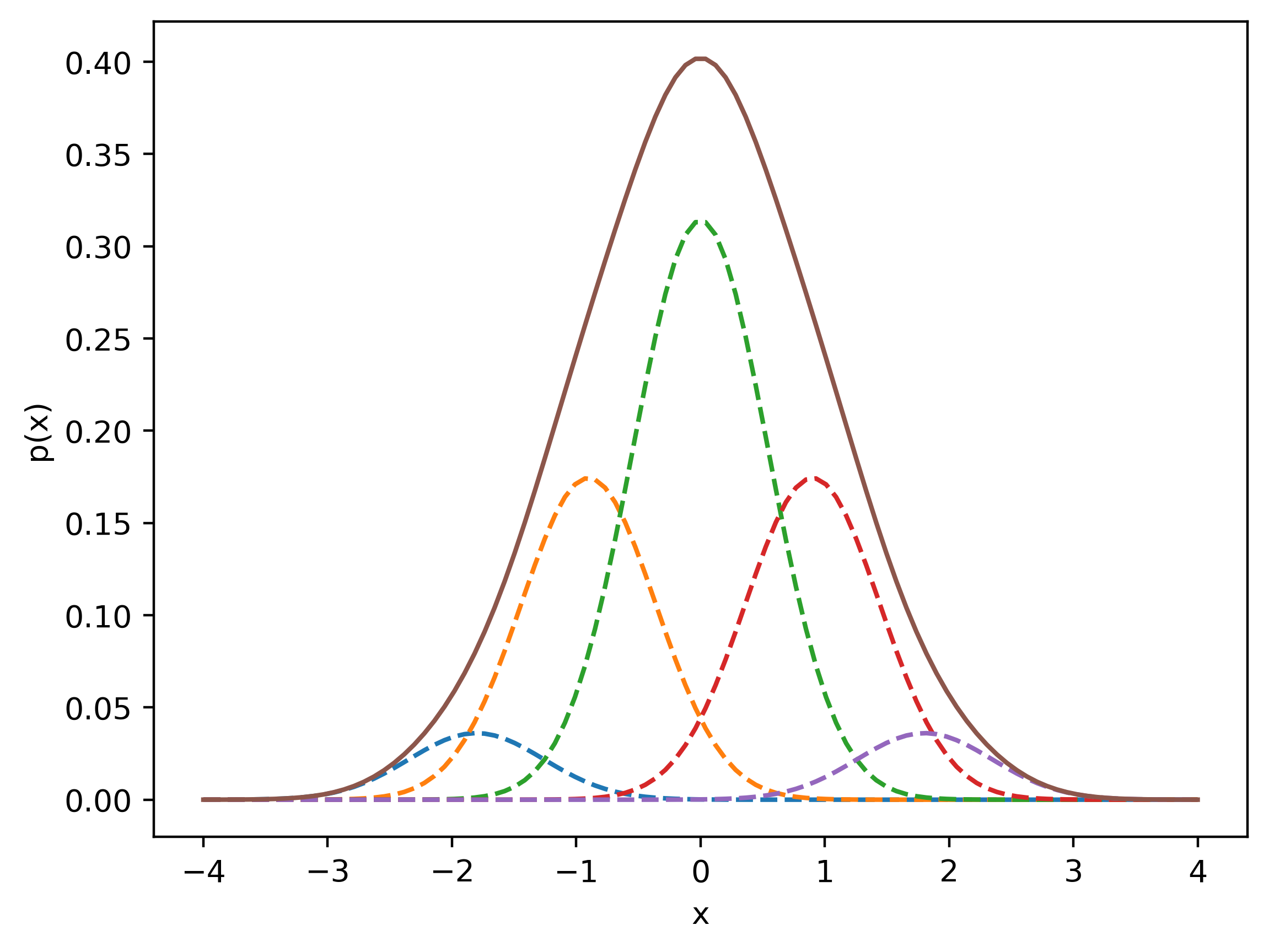
Splitting the Univariate Standard Normal Distribuion
The PyEst library makes it easy to split a univariate standard normal distribution in an optimal way, which is fundamental to the formation of so-called “splitting libraries.”
Each splitting solution is determined by the number of mixands \(L\) and the regularization parameter \(\lambda\), which controls how large the resulting mixand variances are.
The first time PyEst generates an optimal split solution for an \((L,\lambda)\) pair that hasn’t been used before, it will solve an optimization problem and cache the resulting solution to disk. All future calls with this parameter pair will simply reference the cached result and thus be much faster.
import pyest.gm as gm
import matplotlib.pyplot as plt
import numpy as np

# find the optimal standard normal split solutions for different mixture
# sizes and regularization parameter values
L = 5
lam = 1e-3
p = gm.split_1d_standard_gaussian(L, lam)

# we can now plot each of the mixands by using the iterable feature of GaussianMixture
x = np.linspace(-4, 4, 100)
fig, ax = plt.subplots()
for wi, mi, Pi in p:
    ax.plot(x, wi*gm.eval_mvnpdf(x[:, np.newaxis], mi, Pi), linestyle='--')

# plot the GM approximation
ax.plot(x, p(x[:, np.newaxis]), linestyle='-')
ax.set_xlabel('x')
ax.set_ylabel('p(x)')
plt.show()
# # save figure at high resolution with no extra whitespace
# fig.savefig('univariate_split.png', dpi=400, bbox_inches='tight')
Splitting and Plotting PyEst Gaussian Mixtures
This example demonstrates using PyEst to split a mixand in a Gaussian mixture, and how to plot the resulting Gaussian mixture:
# example_2d_gm_split.py
# Written by Keith LeGrand, April 2020
import numpy as np
import matplotlib.pyplot as plt
from pyest import gm

# plot a 2D, 3 component Gaussian mixture
N = 3
# weights
w = np.array([0.4, 0.3, 0.3])
# means
m = np.array([[-0.3, 0.4], [0.1, 1.2], [0.5, 0.4]])
# covariances
P = np.tile(np.diag([0.3**2, 0.2**2]), (N, 1, 1))

# form the Gaussian mixture
gmm = gm.GaussianMixture(w, m, P)
# sample GM on 100x100 grid for plotting
p, X, Y = gmm.pdf_2d(dimensions=[0, 1], res=100)

plt.figure()
plt.contourf(X, Y, p)
# plot the sigma contours of the components
for w, m, P in gmm:
    XY = gm.sigma_contour(m, P, sig_mul=2)
    plt.plot(XY[:, 0], XY[:, 1])

plt.xlabel('$x$')
plt.ylabel('$y$')
plt.show()

# split the first GM component into 3 smaller components
split_options = gm.GaussSplitOptions(L=3, lam=0.001)
split_comp = gm.split_gaussian(*gmm.pop(0), split_options)
gmm += split_comp

# sample GM on 100x100 grid for plotting
p, X, Y = gmm.pdf_2d(dimensions=[0, 1], res=100)

plt.figure()
plt.contourf(X, Y, p)

# plot the sigma contours of the components
for w, m, P in gmm:
    XY = gm.sigma_contour(m, P, sig_mul=2)
    plt.plot(XY[:, 0], XY[:, 1])

plt.xlabel('$x$')
plt.ylabel('$y$')
plt.show()
Gaussian Mixture Splitting for Field-of-View and Negative Information
This example demonstrates recursive splitting for fields-of-view for incorporating negative information:
# %%
from copy import deepcopy

import matplotlib.pyplot as plt
import numpy as np
# %%
import pyest
from pyest import gm
from pyest.sensors.defaults import default_poly_fov

# %%
p = gm.defaults.default_gm(covariance_rotation=np.pi / 6)
fov = default_poly_fov()

# %%
# compute the unnormalized posterior numerically for comparison
pp, XX, YY = p.pdf_2d(dimensions=(0, 1), res=400)
# find which points are inside fov
in_mask = fov.contains(np.vstack((XX.flatten(), YY.flatten())).T)
in_mask_mat = np.reshape(in_mask, XX.shape)
# set pdf evaluations inside fov to zero
pp[in_mask_mat] = 0

# %%
fig = plt.figure()
ax = fig.add_subplot(111)
ax.contourf(XX, YY, pp)
plt.title("Example 1: True Posterior Density")

# %%
split_opts = gm.GaussSplitOptions(L=3, lam=1e-3, min_weight=1e-2)
p_split = gm.split_for_fov(p, fov, split_opts)

# compute the sum of the weights of components outside the FoV
comp_mask_in_fov = np.array(fov.contains(p_split.m[:, :2]))


# %%
p_oofov = gm.GaussianMixture(*p_split[~comp_mask_in_fov])

# %%
pp, xx, yy = p_oofov.pdf_2d(dimensions=(0, 1), res=400)

fig = plt.figure()
ax = fig.add_subplot(111)
ax.contourf(xx, yy, pp, levels=150)
ax.plot(*fov.polygon.exterior.xy)
plt.title("Example 1: Split Density")

fig = plt.figure()
ax = fig.add_subplot(111)
ax.contourf(xx, yy, pp, levels=150)
ax.plot(p_split.m[:, 0], p_split.m[:, 1], '.')
ax.plot(*fov.polygon.exterior.xy)
plt.title("Example 1: Split Density w/ Mixand Mean Locations")

# %%
# -------- Example 2: Two FoVs, pD=0.9 -------------
# create a cone FoV
r = 10
alpha = np.pi / 6
arcx = r * np.cos(np.pi / 2 + np.linspace(-alpha / 2, alpha / 2))
arcy = r * np.sin(np.pi / 2 + np.linspace(-alpha / 2, alpha / 2))
fov_verts = np.vstack(([0, 0], np.vstack((arcx, arcy)).T))
fov = pyest.sensors.PolygonalFieldOfView(fov_verts)

# create a second cone FoV
fov_rot_ang = np.pi / 8
fov_disp = np.array([3, 2])
dcm = np.array([[np.cos(fov_rot_ang), -np.sin(fov_rot_ang)],
                [np.sin(fov_rot_ang), np.cos(fov_rot_ang)]])
fov2 = pyest.sensors.PolygonalFieldOfView(fov_disp + (dcm @ fov_verts.T).T)

# %%
# create a new distribution
m = np.array([0, 5])
cov_ang = np.pi / 5
# rotate the covariance
Py = np.diag([3, 1]) ** 2
dcm = np.array([[np.cos(cov_ang), -np.sin(cov_ang)],
                [np.sin(cov_ang), np.cos(cov_ang)]])
P = dcm @ Py @ dcm.T
w = 1
p_simple = gm.GaussianMixture(w, m, P)

# %%
# plot limits
xlim = [-5, 5]
ylim = [-1, 11]

# %%
pp, xx, yy = p_simple.pdf_2d(dimensions=(0, 1), res=400, xbnd=xlim, ybnd=ylim)
fig = plt.figure()
ax = fig.add_subplot(111)
ax.contourf(xx, yy, pp, levels=150)
ax.plot(*fov.polygon.exterior.xy, color='w')
ax.plot(*fov2.polygon.exterior.xy, color='w')
ax.set_xlim(xlim)
ax.set_ylim(ylim)
ax.set_aspect('equal', adjustable='box')
ax.tick_params(
    axis='both',  # changes apply to both axes
    which='both',  # both major and minor ticks are affected
    bottom=False,  # ticks along the bottom edge are off
    top=False,  # ticks along the top edge are off
    left=False,  # ticks along the left edge are off
    right=False,  # ticks along the right edge are off
    labelbottom=False,  # labels along the bottom edge are off
    labelleft=False)  # labels along the left edge are off
plt.savefig('FigConeFovDensity.png', dpi=300, transparent=True, bbox_inches='tight')
plt.title("Example 2: Prior Density")

# %%
# split the density along the FoV bounds
p_simple_split = gm.split_for_fov(p_simple, [fov, fov2], split_opts)

# specify a probability of detection
pD = 0.9
# update pdf as if no detection inside FoV
p_simp_upd = deepcopy(p_simple_split)
p_simp_upd.w[fov.contains(p_simp_upd.m)] *= (1 - pD)
p_simp_upd.w[fov2.contains(p_simp_upd.m)] *= (1 - pD)

# %%
pp, xx, yy = p_simp_upd.pdf_2d(dimensions=(0, 1), res=400, xbnd=xlim, ybnd=ylim)
fig = plt.figure()
ax = fig.add_subplot(111)
ax.contourf(xx, yy, pp, levels=150)
ax.plot(*fov.polygon.exterior.xy, color='w')
ax.plot(*fov2.polygon.exterior.xy, color='w')
ax.set_xlim(xlim)
ax.set_ylim(ylim)
ax.set_aspect('equal', adjustable='box')
ax.tick_params(
    axis='both',  # changes apply to both axes
    which='both',  # both major and minor ticks are affected
    bottom=False,  # ticks along the bottom edge are off
    top=False,  # ticks along the top edge are off
    left=False,  # ticks along the left edge are off
    right=False,  # ticks along the right edge are off
    labelbottom=False,  # labels along the bottom edge are off
    labelleft=False)  # labels along the left edge are off
plt.savefig('FigConeFovDensitySplitUpdated.png', dpi=300, transparent=True, bbox_inches='tight')
plt.title("Example 2: Split and Updated Posterior, pD=0.9")
plt.show()

# %%
Cartesian to Polar Transformation
This example demonstrates the transformation of a Gaussian mixture from Cartesian to polar coordinates:
import matplotlib as mpl
import matplotlib.pyplot as plt
import numpy as np
import sympy as sp

import pyest.gm as pygm
import pyest.gm.split as split
from pyest.filters.sigma_points import SigmaPointOptions, unscented_transform
from pyest.gm import GaussianMixture
from pyest.linalg import triangularize


# plotting functions
mpl.rcParams.update({
    'font.family': 'serif',
    'text.usetex': True,
})


def bounds_from_meshgrids(XX1, YY1, XX2, YY2):
    x_max = np.max(np.concatenate([XX1.ravel(), XX2.ravel()]))
    x_min = np.min(np.concatenate([XX1.ravel(), XX2.ravel()]))
    y_max = np.max(np.concatenate([YY1.ravel(), YY2.ravel()]))
    y_min = np.min(np.concatenate([YY1.ravel(), YY2.ravel()]))
    return x_min, x_max, y_min, y_max


def save_figure(example, split_method, ax, fig, w=3, h=3):
    # save title text before clearing the title
    title_text = ax.get_title()
    ax.set_title('')
    fig.set_size_inches(w=w, h=h)
    filename = example + split_method.replace(' ', '_')
    fig.savefig(filename + '.svg', bbox_inches='tight', pad_inches=0)
    ax.set_title(title_text)


def plot_split_and_transformed(p_split, py, split_method_str, example, dims=(0, 1),
                               scatter_means=True, xf_lim=None, yf_lim=None, ax_equal=False):
    num_contours = 100
    scatter_plt_args = {'marker': 'x', 'zorder': 2, 'color': 'k'}
    scatter_plt_overlay_args = {'s': 5**2, 'marker': 'x',
                                'zorder': 2.1, 'color': 'w', 'alpha': 0.9, 'linewidth': 1}
    # Plot the split density
    pp, XX, YY = p_split.pdf_2d(res=300, dimensions=dims)
    plt.figure()
    plt.contour(XX, YY, pp, num_contours)
    plt.title('Original Density, split,  ' + split_method_str, wrap=True)
    plt.colorbar()
    if scatter_means:
        plt.scatter(p_split.m[:, dims[0]],
                    p_split.m[:, dims[1]], **scatter_plt_args)
        plt.scatter(p_split.m[:, dims[0]], p_split.m[:,
                    dims[1]], **scatter_plt_overlay_args)
    plt.grid()
    plt.xlabel('$x$')
    plt.ylabel('$y$')

    save_figure(example, split_method_str + "before_map" +
                str(dims), plt.gca(), plt.gcf())

    # Plot the transformed split density
    pp, XX, YY = py.pdf_2d(res=300, dimensions=dims, xbnd=xf_lim, ybnd=yf_lim)
    fig, ax = plt.subplots()
    c = ax.contour(XX, YY, pp, num_contours, linewidths=0.5)
    fig.colorbar(c)
    ax.set_title('Transformed Density, ' + split_method_str, wrap=True)
    if scatter_means:
        ax.scatter(py.m[:, dims[0]], py.m[:, dims[1]], **scatter_plt_args)
        ax.scatter(py.m[:, dims[0]], py.m[:, dims[1]],
                   **scatter_plt_overlay_args)
    ax.grid()
    if xf_lim is not None:
        ax.set_xlim(xf_lim)
    if yf_lim is not None:
        ax.set_ylim(yf_lim)
    if ax_equal:
        ax.set_aspect('equal', adjustable='box')

    ax.set_xlabel('$R$')
    ax.set_ylabel(r'$\theta$')

    save_figure(example, split_method_str + '_' +
                str(dims[0]) + '_' + str(dims[1]), plt.gca(), plt.gcf())

    pp, XX, YY = py.pdf_2d(res=300, dimensions=dims)
    return pp, XX, YY


# square root EKF propagation for individual mixands
def transform_density_ekf(p_split, ny, g, G):
    my = np.zeros((len(p_split), ny))
    Sy = np.zeros((len(p_split), ny, ny))
    for i in range(len(p_split)):
        my[i] = g(p_split.m[i])
        Gval = G(*p_split.m[i])
        Sy[i] = triangularize(Gval @ p_split.Schol[i])

    wy = p_split.w.copy()
    return GaussianMixture(wy, my, Sy, cov_type='cholesky')


# density propagation example in the Cartesian to Polar transformation
def cartesian_to_polar_example():
    example = 'cart2polar'
    # Define the transformation from Cartesian to Polar coordinates
    def cartesian_to_polar(x): return [np.sqrt(
        x[0]**2 + x[1]**2), np.arctan2(x[1], x[0])]
    # Define the transformation from Polar to Cartesian coordinates
    def polar_to_cartesian(y): return [y[0]*np.cos(y[1]), y[0]*np.sin(y[1])]
    ny = 2  # dimension of y
    nx = 2  # dimension of x
    # some limits for integration
    theta_max = 2*np.pi
    theta_min = 0

    # Define the Gaussian mixture
    weights = np.array([1])  # single component
    means = np.array([[0, 1000]])  # 2D in Cartesian coordinates
    covariances = 250**2*np.array([[[16, 0], [0, 1]]])  # covariance matrix
    # we'll use GM even though we only have a single component for generality
    p0 = GaussianMixture(weights, means, covariances)

    # ---- true density plotting ----
    # the true transformed density can be found in terms of the determinant of the inverse mapping
    # can be employed as a reference for GMM propagation
    def py_true(y): return 0 if y[0] < 0 else y[0]*p0(polar_to_cartesian(y))

    # Define the unscented transform parameters
    sigma_pt_opts = SigmaPointOptions(alpha=1e-3, beta=2, kappa=0)
    # Compute the unscented transform of the Gaussian mixture
    mean_polar, covariance_polar, Dt, sigmas, my = unscented_transform(
        p0.m[0], p0.P[0], cartesian_to_polar, sigma_pt_opts=sigma_pt_opts)

    # Create a Gaussian mixture for the transformed density
    p0_polar = GaussianMixture(
        weights, mean_polar, covariance_polar, cov_type='full')

    # Plot the original density
    pp, XX, YY = p0.pdf_2d()
    plt.figure()
    plt.contour(XX, YY, pp, 100)
    plt.title('Original Density')
    plt.xlabel('$x$')
    plt.ylabel('$y$')

    # Plot the true transformed density
    # for laziness, use the linear transformation to generate grid points
    _, XX_true, YY_true = p0_polar.pdf_2d()
    pp_true = np.array([py_true([x, y]) for x, y in zip(
        XX_true.ravel(), YY_true.ravel())]).reshape(XX_true.shape)
    fig, ax = plt.subplots()
    c = ax.contour(XX_true, YY_true, pp_true, 100, linewidths=0.5)
    ax.set_title('True Transformed Density')
    ax.set_xlabel('$R$')
    ax.set_ylabel(r'$\theta$')
    fig.colorbar(c)

    # plt.gca().set_aspect('equal', adjustable='box')
    # Grab the limits
    x_lim = ax.get_xlim()
    y_lim = ax.get_ylim()
    ax.grid()
    save_figure(example, 'truth', plt.gca(), plt.gcf(), w=3, h=3)

    # GMM splitting based density propagation
    # Define the Cartesian to Polar conversion in sympy
    x, y = sp.symbols('x y')
    r = sp.sqrt(x**2 + y**2)
    theta = sp.atan2(y, x)
    cartesian_to_polar_sym = sp.Matrix([r, theta])

    # Compute the symbolic Jacobian
    jacobian = cartesian_to_polar_sym.jacobian([x, y])

    # Compute the symbolic Hessian
    hessian = [sp.hessian(cartesian_to_polar_sym[i], [x, y])
               for i in range(nx)]

    # Lambdify the Jacobian and Hessian
    jacobian_func = sp.lambdify([x, y], jacobian)
    hessian_func = sp.lambdify([x, y], hessian)

    # compare the different split directions
    split_opts = pygm.GaussSplitOptions(
        L=3, lam=1e-3, recurse_depth=2, min_weight=1e-5)

    recursive_split_args = {}
    # use the same number of recursive splits for each mixand
    split_tol = -np.inf
    # settings for the SADL and ALoDT based metrics
    diff_stat_det_sigma_pt_opts = SigmaPointOptions(
        alpha=0.5)  # spread sigma points farther

    # define parameters associated with each splitting method
    # two equally performing methods
    recursive_split_args['variance'] = (split.id_variance, split_tol)
    recursive_split_args['WUSSOLC'] = (
        split.id_wussolc, hessian_func, jacobian_func, split_tol)
    # a method that does not perform as well in this non-dynamical context
    recursive_split_args['USFOS'] = (split.id_usfos, jacobian_func, split_tol)

    # plot the results for each splitting method
    for split_method, args in recursive_split_args.items():
        p_split = split.recursive_split(p0, split_opts, *args)
        py = transform_density_ekf(
            p_split, ny, cartesian_to_polar, jacobian_func)
        _, XX, YY = plot_split_and_transformed(
            p_split, py, split_method, example, xf_lim=x_lim, yf_lim=y_lim)

    plt.show()


if __name__ == '__main__':
    # run the example
    cartesian_to_polar_example()
Cislunar Space Object Uncertainty Propagation
This example shows how to use pyest for propagating uncertainty in the circular restricted three-body problem (CR3BP).
Note
This example utilizes a cache of precomputed Monte Carlo samples to evaluate various performance measures. If the cache is not available, this example will generate new samples and store them in a cache for future use. On first run, this may take a few minutes to build the cache. These samples are only for performance evaluation and not required for any of the adaptive Gaussian splitting operations.
import matplotlib as mpl
import matplotlib.pyplot as plt
import numpy as np
from STMint.STMint import STMint
from diskcache import Cache

import pyest.gm as pygm
import pyest.gm.split as split
from pyest.filters.sigma_points import SigmaPointOptions
from pyest.gm import GaussianMixture
from pyest.linalg import triangularize


# plotting functions
mpl.rcParams.update({
    'font.family': 'serif',
    'text.usetex': True,
})


def bounds_from_meshgrids(XX1, YY1, XX2, YY2):
    x_max = np.max(np.concatenate([XX1.ravel(), XX2.ravel()]))
    x_min = np.min(np.concatenate([XX1.ravel(), XX2.ravel()]))
    y_max = np.max(np.concatenate([YY1.ravel(), YY2.ravel()]))
    y_min = np.min(np.concatenate([YY1.ravel(), YY2.ravel()]))
    return x_min, x_max, y_min, y_max


def save_figure(example, split_method, ax, fig, w=3, h=3):
    # save title text before clearing the title
    title_text = ax.get_title()
    ax.set_title('')
    fig.set_size_inches(w=w, h=h)
    filename = example + split_method.replace(' ', '_')
    fig.savefig(filename + '.svg', bbox_inches='tight', pad_inches=0)
    ax.set_title(title_text)


def plot_split_and_transformed(p_split, py, split_method_str, example, dims=(0, 1),
                               scatter_means=True, xf_lim=None, yf_lim=None, ax_equal=False):
    num_contours = 100
    scatter_plt_args = {'marker': 'x', 'zorder': 2, 'color': 'k'}
    scatter_plt_overlay_args = {'s': 5**2, 'marker': 'x',
                                'zorder': 2.1, 'color': 'w', 'alpha': 0.9, 'linewidth': 1}
    # Plot the split density
    pp, XX, YY = p_split.pdf_2d(res=300, dimensions=dims)
    plt.figure()
    plt.contour(XX, YY, pp, num_contours)
    plt.title('Original Density, split,  ' + split_method_str, wrap=True)
    plt.colorbar()
    if scatter_means:
        plt.scatter(p_split.m[:, dims[0]],
                    p_split.m[:, dims[1]], **scatter_plt_args)
        plt.scatter(p_split.m[:, dims[0]], p_split.m[:,
                    dims[1]], **scatter_plt_overlay_args)
    plt.grid()
    labels = ['$x$', '$y$', '$z$', r'$\dot{x}$', r'$\dot{y}$', r'$\dot{z}$']
    plt.xlabel(labels[dims[0]])
    plt.ylabel(labels[dims[1]])

    save_figure(example, split_method_str + "before_map" +
                str(dims), plt.gca(), plt.gcf())

    # Plot the transformed split density
    pp, XX, YY = py.pdf_2d(res=300, dimensions=dims, xbnd=xf_lim, ybnd=yf_lim)
    fig, ax = plt.subplots()
    c = ax.contour(XX, YY, pp, num_contours, linewidths=0.5)
    fig.colorbar(c)
    ax.set_title('Transformed Density, ' + split_method_str, wrap=True)
    if scatter_means:
        ax.scatter(py.m[:, dims[0]], py.m[:, dims[1]], **scatter_plt_args)
        ax.scatter(py.m[:, dims[0]], py.m[:, dims[1]],
                   **scatter_plt_overlay_args)
    ax.grid()
    if xf_lim is not None:
        ax.set_xlim(xf_lim)
    if yf_lim is not None:
        ax.set_ylim(yf_lim)
    if ax_equal:
        ax.set_aspect('equal', adjustable='box')

    labels = ['$x$', '$y$', '$z$', r'$\dot{x}$', r'$\dot{y}$', r'$\dot{z}$']
    ax.set_xlabel(labels[dims[0]])
    ax.set_ylabel(labels[dims[1]])

    save_figure(example, split_method_str + '_' +
                str(dims[0]) + '_' + str(dims[1]), plt.gca(), plt.gcf())

    pp, XX, YY = py.pdf_2d(res=300, dimensions=dims)
    return pp, XX, YY
# end plotting utilities


# square root EKF propagation for individual mixands
def transform_density_ekf(p_split, ny, g, G):
    my = np.zeros((len(p_split), ny))
    Sy = np.zeros((len(p_split), ny, ny))
    for i in range(len(p_split)):
        my[i] = g(p_split.m[i])
        Gval = G(*p_split.m[i])
        Sy[i] = triangularize(Gval @ p_split.Schol[i])

    wy = p_split.w.copy()
    return GaussianMixture(wy, my, Sy, cov_type='cholesky')


# density propagation example in a Cislunar NRHO
def cislunar_example():
    example = 'cislunar'
    # nrho ics
    mu = 1.0 / (81.30059 + 1.0)
    x0 = 1.02202151273581740824714855590570360
    z0 = -0.182096761524240501132977765539282777
    yd0 = -0.103256341062793815791764364248006121
    period = 1.5111111111111111111111111111111111111111
    transfer_time = period * 0.5

    x_0 = np.array([x0, 0, z0, 0, yd0, 0])
    ny = 6  # dimension of y
    nx = 6  # dimension of x

    weights = np.array([1])  # single component
    cov_0 = 0.00001**2 * np.identity(6) + \
        0.0001**2 * (np.diag([1, 0, 1, 0, 0, 0]))
    p0 = GaussianMixture(weights, np.array([x_0]), np.array([cov_0]))

    # nrho propagator
    integrator = STMint(preset="threeBody", preset_mult=mu,
                        variational_order=2)
    max_integrator_step = period/500.0
    int_tol = 1e-13

    # outputs x_f, STM, STT
    def flow_info(x, y, z, vx, vy, vz): return integrator.dynVar_int2(
        [0, transfer_time], [x, y, z, vx, vy, vz], rtol=int_tol, atol=int_tol, output="final"
    )
    # outputs just the hessian

    def hessian_func(x, y, z, vx, vy, vz): return integrator.dynVar_int2(
        [0, transfer_time], [x, y, z, vx, vy, vz], rtol=int_tol, atol=int_tol, output="final"
    )[2]
    # outputs just the jacobian

    def jacobian_func(x, y, z, vx, vy, vz): return integrator.dynVar_int(
        [0, transfer_time], [x, y, z, vx, vy, vz], rtol=int_tol, atol=int_tol, output="final"
    )[1]
    # outputs flow of state only

    def propagation(x_0): return integrator.dyn_int([0, transfer_time], x_0,
                                                    max_step=max_integrator_step,
                                                    t_eval=[transfer_time]).y[:, -1]

    # apply splitting methods
    split_opts = pygm.GaussSplitOptions(
        L=3, lam=1e-3, recurse_depth=3, min_weight=-np.inf)

    # Define the unscented transform parameters
    sigma_pt_opts = SigmaPointOptions(alpha=1e-3, beta=2, kappa=0)

    print("running monte carlo")
    # create/load split cache
    cislunar_mc_cache = Cache(__file__[:-3] + 'cislunar_mc_cache')
    # reference Monte Carlo (store points and pdf value at point)
    num_points = int(1e4)
    rng = np.random.default_rng(100)
    if 'samples' in cislunar_mc_cache:
        print("cache found, loading samples from cache")
        samples = cislunar_mc_cache['samples']
        final_samples = cislunar_mc_cache['final_samples']
        assert (len(samples) == num_points)
    else:
        print("cache not found, propagating samples")
        samples = rng.multivariate_normal(x_0, cov_0, num_points)
        final_samples = list(map(propagation, samples))
        cislunar_mc_cache['samples'] = samples
        cislunar_mc_cache['final_samples'] = final_samples
        print("MC propagation complete, cache saved with {} samples".format(num_points))

    idx_pairs = [(0, 1), (0, 2), (1, 2), (3, 4),
                 (4, 5), (3, 5), (0, 4), (1, 3)]
    axis_labels = ['$x$', '$y$', '$z$',
                   r'$\dot{x}$', r'$\dot{y}$', r'$\dot{z}$']

    # scatter plotting for Monte Carlo
    xlim = dict()
    ylim = dict()
    for idx_pair in idx_pairs:
        plt.figure()
        plt.scatter(np.array(final_samples)[:, idx_pair[0]], np.array(
            final_samples)[:, idx_pair[1]], marker='+', alpha=0.025)
        plt.xlabel(axis_labels[idx_pair[0]])
        plt.ylabel(axis_labels[idx_pair[1]])
        save_figure(example, "truth_scatter" + '_' +
                    str(idx_pair[0]) + '_' + str(idx_pair[1]), plt.gca(), plt.gcf())
        plt.figure()
        plt.hist2d(np.array(final_samples)[:, idx_pair[0]], np.array(
            final_samples)[:, idx_pair[1]], 40)
        plt.xlabel(axis_labels[idx_pair[0]])
        plt.ylabel(axis_labels[idx_pair[1]])
        # save axis limits for later
        xlim[idx_pair] = plt.gca().get_xlim()
        ylim[idx_pair] = plt.gca().get_ylim()
        save_figure(example, "truth_hist" + '_' +
                    str(idx_pair[0]) + '_' + str(idx_pair[1]), plt.gca(), plt.gcf())

    recursive_split_args = {}
    # use the same number of recursive splits for each mixand
    split_tol = -np.inf
    # settings for the SADL and ALoDT based metrics
    diff_stat_det_sigma_pt_opts = SigmaPointOptions(
        alpha=0.5)  # spread sigma points farther

    # define parameters associated with each splitting method
    recursive_split_args['variance'] = (split.id_variance, split_tol)
    recursive_split_args['USFOS'] = (split.id_usfos, jacobian_func, split_tol)
    recursive_split_args['WUSSADL'] = (
        split.id_wussadl, jacobian_func, propagation, diff_stat_det_sigma_pt_opts, split_tol)
    recursive_split_args['WUSSOLC'] = (
        split.id_wussolc, hessian_func, jacobian_func, split_tol)

    # additional splitting methods
    # uncomment these if desired
    # recursive_split_args['ALoDT'] = (split.id_max_alodt, propagation, diff_stat_det_sigma_pt_opts, split_tol)
    # recursive_split_args['FOS'] = (split.id_fos, jacobian_func, split_tol)
    # recursive_split_args['SAFOS'] = (split.id_safos, jacobian_func, split_tol)
    # recursive_split_args['USFOS'] = (split.id_usfos, jacobian_func, split_tol)
    # recursive_split_args['SOS'] = (split.id_sos, hessian_func, jacobian_func, split_tol)
    # recursive_split_args['SASOS'] = (split.id_sasos, hessian_func, split_tol)
    # recursive_split_args['WSASOS'] = (split.id_wsasos, hessian_func, jacobian_func, split_tol)
    # recursive_split_args['WUSSOS'] = (split.id_wussos, hessian_func, jacobian_func, split_tol)
    # recursive_split_args['SOLC'] = (split.id_solc, hessian_func, split_tol)
    # recursive_split_args['USSOLC'] = (split.id_ussolc, hessian_func, split_tol)
    # recursive_split_args['SADL'] = (split.id_sadl, jacobian_func, propagation, diff_stat_det_sigma_pt_opts, split_tol)

    # plot the resulting GMM densities propagated
    for split_method, args in recursive_split_args.items():
        p_split = split.recursive_split(p0, split_opts, *args)
        py = transform_density_ekf(p_split, ny, propagation, jacobian_func)

        for idx_pair in idx_pairs:
            _, XX, YY = plot_split_and_transformed(
                p_split, py, split_method, example, idx_pair, xf_lim=xlim[idx_pair], yf_lim=ylim[idx_pair])

    plt.show()


if __name__ == '__main__':
    # run the example
    cislunar_example()